The Data Science team at Greenhouse Group is steadily growing and continuously changing. This also implies new Data Scientists and interns starting regularly. Each new Data Scientist we hire is unique and has a different set of skills. What they all have in common though is a strong analytical background and the practical ability to apply this on real business cases. The majority of our team for example studied Econometrics, a study which provides a strong foundation in probability theory and statistics.
As the typical Data Scientist also has to work with lots of data, decent programming skills are a must-have. This is however where the backgrounds of our new Data Scientists tends to differ from each other. The programming landscape is quite diverse, and therefore, the backgrounds of our new Data Scientists cover programming languages from R, MatLab, Java, Python, STATA, SPSS, SAS, SQL, Delphi, PHP to C# and C++. It is true that knowing many different programming languages can be useful when necessary. However, we prefer the use of one language for the majority of our projects so that we can easily cooperate with each other on projects. And given that nobody knows everything, one preferred programming language gives us the possibility to learn from each other.
At Greenhouse Group we have chosen to work with Python when possible. With the great support of the open-source community, Python has transformed into a great tool for doing Data Science. Python’s easy to use syntax, great data processing capabilities and awesome open-source statistical libraries such as Numpy, Pandas, Scikit-learn and Statsmodels allow us to do a wide range of tasks varying from exploratory analysis to building scalable big-data pipelines and machine learning algorithms. Only for the lesser-general statistical models we sometimes combine Python with R, where Python does the heavy data processing work and R the statistical modelling.
I also strongly believe in the philosophy of learning by doing. Therefore, to help our new Data Scientists get on their way with doing Data Science in Python we have created a Python Data Science (Crash) Course. The goal of this course is to let our new recruits (and also colleagues from different departments) learn to solve a real business problem in an interactive way and in their own pace . Meanwhile, the more experienced Data Scientists are available to answer any questions. Note that the skill of Googling for answers on StackOverflow or browsing through the documentation of libraries should not be underestimated. We definitely want to teach our new Data Scientists this skill too!
In this blog we describe our practical course phase by phase.
Phase 1: Learning Python, the basics
The first step obviously is learning Python. That is, learning the Python syntax and basic Python operations. Luckily, the Python syntax is not that difficult if you take good care of indentation. Personally, coming from the Java programming language where indentation is not important, I made a lot of mistakes with indentation when I started with Python.
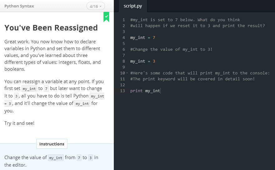
So, how to start with learning Python? Well, as we prefer the learning by doing approach we always let our new recruits start with the Codecademy Python course. Codecademy provides an interactive Python course which can be followed in the browser. Therefore, you do not have to worry about installing anything yet and you can start immediately with learning Python!
The Codecademy Python course takes about 13 hours to complete. After this, you should be able to do simple operations in Python.
Update: I just discovered that Codecademy will temporarily take the Python course offline. I haven’t tried it yet, but a possible alternative to learn Python from within the browser is learnpython.org
Bonus tip: another useful Codecademy course for Data Scientists is the SQL course!

Phase 2: Installing Python locally with Anaconda
After finishing the Codecademy course we obviously want to start developing our own codes. However, since we are not running Python in-browser anymore we need to install Python on our own local PC.
Python is open source and freely available from www.python.org. However, this official version only contains the standard Python libraries. The standard libraries contain functions to work with for example text files, datetimes and basic arithmetic operations. Unfortunately, the standard Python libraries are not comprehensive enough to perform all kinds of Data Science analysis. Luckily, the open-source community has made awesome libraries to extend Python with the proper functionality to do Data Science.
To prevent downloading and installing all these libraries separately, we prefer to use the Anaconda Python distribution. Anaconda is actually Python combined with tons of scientific libraries, so there is no need to manually install them all yourself! Additionally, Anaconda comes bundled with an easy commandline tool to install new or update existing libraries when necessary.
Tip: although allmost all awesome libraries are included by default in Anaconda, some of them are not yet. You can install new packages from the command line using conda install package_name or pip install package_name. For example, we regularly use the progressbar library tqdm in our projects. Hence, we have to execute pip install tqdm first when performing a new install of Anaconda.

Phase 3: Easier coding with PyCharm
After installing Python we are able to run Python code on our local PC. Just start Notepad, write your Python code, open the commandline and run the newly created Python file using python C:\Users\thom\new_file.py. Wait, that does not sound really simple right? No…
To make our lifes easier, we prefer to develop our Python codes in Pycharm. PyCharm is a so-called integrated development environment which supports developers when writing code. It takes care of routine tasks such as running a program by providing a simple run script button. Additionally, it also helps being more productive by providing autocomplete functionality and on-the-fly error checking. Forgot a space somewhere or used a variable name that is not defined yet? PyCharm will warn you. Want to use a Version Control System such as Git to cooperate on projects? PyCharm will help you. One way or another, using PyCharm will save you a lot of time when writing Python code, because it works like a charm… badum tss.

Phase 4: Solving a fictional business problem
Defining the research problem
So, assume that by now our manager has come to us with a business problem he faces.
That is, our manager wants to be able to predict the probability of a user having his first engagement (i.e. a newsletter subscription) on the companies website. After giving it some thought we came up with the idea to predict the engagement conversion probability based on his number of pageviews. Furthermore, you constructed the following hypothesis:
More pageviews leads to a higher probability of engaging for the first time.
To check whether this hypothesis holds, we have asked our Web Analysts for two datasets:
- Session data containing all pageviews of all users.
user_id: a unique user identifiersession_number: the number of the sessions (ascending)session_start_date: the start datetime of the sessionunix_timestamp: the start unix timestamp of the sessioncampaign_id: ID of the campaign that led the user to the websitedomain: the (sub)domain the user is visiting in this sessionentry: the entry page of the sessionreferral: the referring site, i.e. google.compageviews: the number of pageviews within the sessiontransactions: the number of transactions within the session
- Engagement data containing all engagements of all users
user_id: a unique user identifiersite_id: the ID of the site on which the engagement took placeengagement_unix_timestamp: the unix timestamp of when the engagement took placeengagement_type: the type of engagement, i.e. newsletter subscriptioncustom_properties: additional properties of the engagement
Unfortunately, we have two separate datasets because they come from different systems. However, users in both datasets can be matched by a unique user identifier denoted by user_id.
Just like earlier blogs, I have placed the final code to solve the business problem on my GitHub. However, I would strongly recommend to only look at this code when you have solved the case yourself. Additionally, you can also find the code to create two fictional datasets yourself.
Easy data processing using Pandas
Before we can apply any statistical model to solve the problem we need to clean and prepare our data. For example, we need to find for each user in the sessions dataset his first engagement, if any. This requires joining the two datasets on user_id and removing any engagements after the first.
The Codecademy Python course taught you already how to read text files line by line. Python is great for data munging and preparation, but not for data analysis and modeling. The Pandas library for Python helps to overcome this problem. Pandas offers data structures and operations for manipulating (numerical) tables and time series. Pandas therefore makes it much easier to do Data Science in Python!

Reading the datasets using pd.read_csv()
The first step in our Python code will be to load both datasets within Python. Pandas provides an easy to use function to read .csv files: read_csv(). Following the learning by doing principle we recommend you find out yourself how to read both datasets. In the end, you should have two separate DataFrames, one for each dataset.
Tips: we have different delimiters in both files. Also, be sure to check out the date_parser option in read_csv() to convert the UNIX timestamps to normal datetime formats.
Filter out irrelevant data
The next step in any (big) data problem is to reduce the size of your problem. In our case, we have lots of columns which are not relevant for our problem, such as the medium/source of the session. Therefore, we apply Indexing and Selecting on our Dataframes to only keep relevant columns such as the user_id (necessary to join the two DataFrames), datetimes of each session and engagement (to search for the first engagement and sessions before that) and the number of pageviews (necessary to test our hypothesis).
Additionally, we filter out all non-first engagements in our engagements DataFrame. This can be done by looking for the lowest datetime value for each user_id. How? Use the GroupBy: split-apply-combine logic! 🙂
Combine the DataFrames based on user_id
One of the most powerful options of Pandas is merging, joining and concatenating tables. It allows us to perform anything from simple left joins and unions to complex full outer joins. SO, combining the sessions and first engagements DataFrames based on the unique user identifier… you’ve got the power!
Remove all sessions after the first engagement
Using a simple merge in the previous step we added to each session the timestamp of the first engagement. By comparing the session timestamp with the first engagement timestamp you should be able to filter out irrelevant data and reduce the size of the problem as well.
Add the dependent variable y: an engagement conversion
As stated, we want to predict the effect of pageviews on the conversion (i.e. first engagement) probability. Therefore, our dependent y variable is a binary variable which denotes whether a conversion has taken place within the session. Because of the filtering we did above (i.e. remove all non-first engagements and sessions after te first engagement), this conversion by definition takes place in the last session of each user. Again, using the GroupBy: split-apply-combine logic we can create a new column that contains a 1-observation if it is the last sessions of a user, and a 0-observation otherwise.
Add the independent variable X: cumulative sum of pageviews
Our independent variable is the number of pageviews. However, we cannot simply take the number of pageviews within a session, because pages visited in earlier sessions can also affect the conversion probability. Hence, we create a new column in which we calculate the cumulative sum of pageviews for a user. This will be our independent variable X.
Fit a logistic regression using StatsModels
Using Pandas we finally ended up with a small DataFrame containing of a single discrete X column and a single binary y column. A (binary) logistic regression model is used to estimate the probability of a binary response of the dependent variable based on one or more independent variables. StatsModels is a statistics & econometrics libary for Python with tools for parameter estimation & statistical testing. Therefore it is not surprising that it also contains functions to perform a logistic regression. So, how to fit a Logistic regression model using StatsModels? Let me Google that for you!
Tip 1: do not forget to add a constant to the logistic regression…
Tip 2: another awesome libary to fit statistical models such as logistic regression is scikit-learn.

Visualize results using Matplotlib or Seaborn
After fitting the logistic regression model, we can predict the conversion probability for each cumulative pageviews value. However, we cannot just communicate our newly found results to the management by handing over some raw numbers. Therefore, one of the important tasks of a Data Scientist is to present his results in a clearly and effective manner. In most cases, this means providing visualizations of our results as we all know that an image is worth more than a thousand words…
Python contains several awesome visualization libraries of which MatplotLib is the most well-known. Seaborn is another awesome libary built upon MatplotLib. The syntax of MatplotLib is probably well-known to users who worked with MatLab before. However, our preference goes to Seaborn as it provides prettier plots and appearance is important.
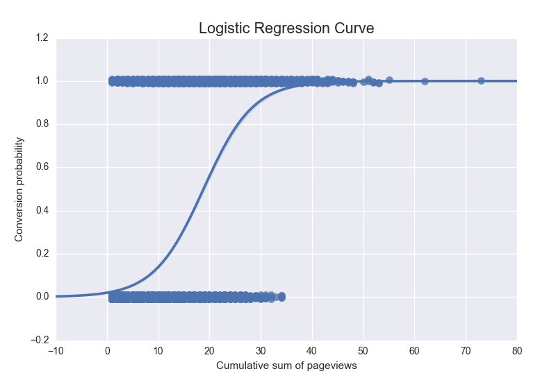
Using Seaborn we created the following visualization of our fitted model:

We can nicely use this visualization to support our evidence on whether our hypothesis holds.
Testing the hypothesis
The final step is to check whether our constructed hypothesis holds. Recall that we stated that
More pageviews leads to a higher probability of engaging for the first time.
For one, from our previous visualization it already follows that the hypothesis holds. Otherwise, the predicted probabilities would not be monotonically increasing. Nonetheless, we could also draw the same conclusion from the summary of our fitted model as shown below.
                           Logit Regression Results
  ==============================================================================
  Dep. Variable:          is_conversion   No. Observations:                12420
  Model:                          Logit   Df Residuals:                    12418
  Method:                           MLE   Df Model:                            1
  Date:                Tue, 27 Sep 2016   Pseudo R-squ.:                  0.3207
  Time:                        21:44:57   Log-Likelihood:                -5057.6
  converged:                       True   LL-Null:                       -7445.5
                                          LLR p-value:                     0.000
  ====================================================================================
                         coef    std err          z      P>|z|      [95.0% Conf. Int.]
  ------------------------------------------------------------------------------------
  const               -3.8989      0.066    -59.459      0.000        -4.027    -3.770
  pageviews_cumsum     0.2069      0.004     52.749      0.000         0.199     0.215
  ====================================================================================
We see that the coefficient of the pageviews_cumsum is statistically significant positive at a significance level of 1%. Hence, we have shown that our hypothesis holds, hurray! Furthermore, you just completed your first Data Science analysis in Python! 🙂
Conclusion
We hope you have enjoyed this Data Science in Python blog. What we described in this blog is obviously far from comprehensive or complete as it is simply too much to cover in one blog. For example, we haven’t even talked about Version Control Systems such as Git yet. We hope however that this blog has given you some directions on how to start with your first practical Data Science analysis in Python. We would appreciate to hear in the comments on how you have set your first steps in Data Science with Python. Also, any valuable feedback to improve this blog or crash course is welcome. 🙂


Leave a Reply
You must be logged in to post a comment.