
A key focus of our Data Science team is to help our clients understand how their marketing spend affects their KPIs. In particular, we create models to understand the effect of individual marketing channels such as television or paid search ads on KPIs such as sales, visits and footfall. Knowing how marketing spend affects KPIs enables us to optimize the clients marketing spend for maximal result. In this Geek post I will give a fictional example on how we use S-curves to optimize radio spend. The final code of this fictional example can be found on Github as well.
The data
Let’s consider a simple example where we have the number of sales and the number of radio GRPs on a daily basis. We assume that radio only has an immediate positive effect on the number of sales the same day. This is obviously not true in real-life, because radio still shows a positive effect after several days. For now, such delayed effects are out of the scope of this post. The figure below provides an overview of how our fictional sales and radio dataset looks like. We see that in this example dataset there are two important factors that determine the number of sales on a day: the day of the week (seasonality) and the number of radio GRPs on that day (marketing spend).

Simple OLS regression
As we are interested in how radio affects the number of sales, we run a simple OLS regression to capture the relationship of marketing spend and seasonality on sales. The results of this regression are shown in the table below.
                            OLS Regression Results
  ==============================================================================
  Dep. Variable:                  sales   R-squared:                       0.920
  Model:                            OLS   Adj. R-squared:                  0.896
  Method:                 Least Squares   F-statistic:                     38.01
  Date:                Thu, 23 Apr 2015   Prob (F-statistic):           3.62e-11
  Time:                        15:00:50   Log-Likelihood:                -47.424
  No. Observations:                  31   AIC:                             110.8
  Df Residuals:                      23   BIC:                             122.3
  Df Model:                           7
  Covariance Type:            nonrobust
  ========================================================================================
                             coef    std err          t      P>|t|      [95.0% Conf. Int.]
  ----------------------------------------------------------------------------------------
  const                    7.4642      0.583     12.793      0.000         6.257     8.671
  radio_grp                1.1423      0.096     11.854      0.000         0.943     1.342
  seasonality_monday      -2.7826      0.820     -3.392      0.003        -4.480    -1.085
  seasonality_tuesday     -0.4115      0.869     -0.473      0.640        -2.210     1.387
  seasonality_thursday    -4.8585      0.903     -5.381      0.000        -6.726    -2.991
  seasonality_friday      -3.7702      0.886     -4.256      0.000        -5.603    -1.938
  seasonality_saturday    -4.9362      0.886     -5.572      0.000        -6.769    -3.104
  seasonality_sunday      -5.3039      0.872     -6.080      0.000        -7.109    -3.499
  ==============================================================================
  Omnibus:                        0.646   Durbin-Watson:                   1.188
  Prob(Omnibus):                  0.724   Jarque-Bera (JB):                0.739
  Skew:                          -0.265   Prob(JB):                        0.691
  Kurtosis:                       2.461   Cond. No.                         24.1
  ==============================================================================

The result of this regression shows that the day of the week is a very important factor for the number of sales. We used Wednesday as reference day and added binary dummy variables for all other days. Note Wednesday is taken arbitrarily. The coefficients of these day-dummies can be interpreted as the number of sales this day has more (or less) compared to the number of sales on Wednesday (the reference day). For example, the Monday coefficient of –2.8 implies that there are 2.8 less absolute sales on Monday than on Wednesday. So, as all day dummy coefficients are negative, it follows that Wednesday is the best day of the week for the sales.
More interestingly, the result of the regression also gives a positive coefficient of 1.14 for the radio variable. This coefficient can be interpreted as a positive effect of 1.14 additional sales for each radio GRP used. Note that this also implies that the effect of radio is linear, i.e. 1 GRP results in 1.14 additional sales and 5 GRPs results in 5 times 1.14 (=5.7) additional sales.
The S-response curve
In reality, it is not often the case that radio has a linear effect on sales. KPI drivers such as television and radio, but also display and search ads tend to have diminishing returns. Wikipedia provides the following example about diminishing returns:
“A common sort of example is adding more workers to a job, such as assembling a car on a factory floor. At some point, adding more workers causes problems such as workers getting in each other’s way or frequently finding themselves waiting for access to a part. Producing one more unit of output per unit of time will eventually cost increasingly more, due to inputs being used less and less effectively.”
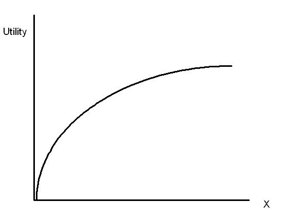
In a similar manner, research has shown that initial advertising budget has little impact on sales. One possible reason for this is that a low advertising budget might result in your marketing not being noticable between all of the competitors marketing campaigns. Only after a certain budget spend threshold results are noticeable in the form of improved KPIs. Hence, the result is that the effect of marketing spend on KPI drivers such as radio typically follows an S-shaped curve. The figure below provides an example of an S-curve for radio spend.

Introducing dummy variables
The notion of the S-shaped curve conflicts with our earlier calculated linear effect of radio on sales. Therefore, it is very likely that we get a much more accurate model when we can account for the effect of the S-curve. One possible approach is to just try all possible transformations of our radio dataset to an S-curve. However, as the S-curve is defined by three parameter values, this implies trying a lot of different transformations. Therefore, we use a smarter approach to find the S-curve. That is, instead of adding a continuous variable that denotes the number of radio GRPs on a given day, we add binary dummies where each dummy represents an interval of GRPs. Given our example dataset where the maximum number of GRPs is 10, we add four binary dummies representing the GRP intervals [0.1-2.4], [2.5-4.9], [5-7.4] and [7.5-10]. Now, the dummy value of an interval is 1 if the number of GRPs of that day is in that interval, otherwise the value is zero. Below is a short snippet of the radio dataset we then obtain:
| Date time | Radio GRP | Radio dummy 0.1 – 2.4 |
Radio dummy 2.5 – 4.9 |
Radio dummy 5.0 – 7.4 |
Radio dummy 7.5 – 10 |
|---|---|---|---|---|---|
| 2015-06-01 | 4 | 0 | 1 | 0 | 0 |
| 2015-06-02 | 0 | 0 | 0 | 0 | 0 |
| 2015-06-03 | 1 | 1 | 0 | 0 | 0 |
| 2015-06-04 | 2 | 1 | 0 | 0 | 0 |
| 2015-06-05 | 3 | 0 | 1 | 0 | 0 |
Using the new radio dummy variables we again run a standard OLS regression. The results of this regression are shown below:
                            OLS Regression Results
  ==============================================================================
  Dep. Variable:                  sales   R-squared:                       0.985
  Model:                            OLS   Adj. R-squared:                  0.978
  Method:                 Least Squares   F-statistic:                     134.6
  Date:                Thu, 23 Apr 2015   Prob (F-statistic):           4.28e-16
  Time:                        15:42:39   Log-Likelihood:                -21.183
  No. Observations:                  31   AIC:                             64.37
  Df Residuals:                      20   BIC:                             80.14
  Df Model:                          10
  Covariance Type:            nonrobust
  ========================================================================================
                             coef    std err          t      P>|t|      [95.0% Conf. Int.]
  ----------------------------------------------------------------------------------------
  const                    8.1073      0.298     27.175      0.000         7.485     8.730
  radio_dummy_0.1_2.5      0.2485      0.334      0.745      0.465        -0.448     0.945
  radio_dummy_2.5_5        1.9554      0.407      4.806      0.000         1.107     2.804
  radio_dummy_5_7.5        8.7667      0.415     21.146      0.000         7.902     9.632
  radio_dummy_7.5_10       9.3869      0.494     19.001      0.000         8.356    10.417
  seasonality_monday      -2.9030      0.405     -7.171      0.000        -3.747    -2.059
  seasonality_tuesday     -0.5771      0.401     -1.439      0.165        -1.413     0.259
  seasonality_thursday    -4.6460      0.430    -10.793      0.000        -5.544    -3.748
  seasonality_friday      -4.3809      0.441     -9.929      0.000        -5.301    -3.461
  seasonality_saturday    -5.2752      0.419    -12.602      0.000        -6.148    -4.402
  seasonality_sunday      -5.9470      0.422    -14.096      0.000        -6.827    -5.067
  ==============================================================================
  Omnibus:                        1.184   Durbin-Watson:                   1.621
  Prob(Omnibus):                  0.553   Jarque-Bera (JB):                0.590
  Skew:                           0.334   Prob(JB):                        0.744
  Kurtosis:                       3.107   Cond. No.                         8.27
  ==============================================================================
The interpretation of the coefficients of the new radio dummy variables is slightly different than in our first regression. The coefficient of each dummy represents the additional sales when the number of GRPs is in the corresponding interval. For example, consider a given day on which 6 radio GRPs are used. This implies that the value of the dummy for the interval [5 – 7.4] is one (and all other dummies are zero) and that this results in an additional 8.5 sales.
| GRP interval | Additional sales |
|---|---|
| 0.1 – 2.4 | 0.3 |
| 2.5 – 4.9 | 2.5 |
| 5 – 7.4 | 8.5 |
| 7.5 – 10 | 10.1 |
Finding the S-curve using the dummy variables
When plotting the additional sales against the GRP intervals we obtain the points in Figure 4. The shape of the S-curve can already be seen in these points. It then is a simple task to find the S-curve that best fits these points. Note that in our example the S-curve we predicted fits the true S-curve (which we used for creating our fictional dataset) quite good because it is nearly the same logistic function. The small difference in curves can be explained due to the fact that we added noise to our fictional dataset to simulate reality.

Final results
So, since we found our best S-curve transformation, we run the first OLS regression again but this time with our radio data transformed to fit the new S-curve. The resulted predictions of the model are plotted in Figure 5. Note that this regression now fits our dataset much better than the first regression we run. Therefore, we are able to obtain much better predictions of the effect of radio on sales! 🙂
                            OLS Regression Results
  ==============================================================================
  Dep. Variable:                  sales   R-squared:                       0.987
  Model:                            OLS   Adj. R-squared:                  0.984
  Method:                 Least Squares   F-statistic:                     258.4
  Date:                Thu, 23 Apr 2015   Prob (F-statistic):           2.56e-20
  Time:                        16:38:53   Log-Likelihood:                -18.808
  No. Observations:                  31   AIC:                             53.62
  Df Residuals:                      23   BIC:                             65.09
  Df Model:                           7
  Covariance Type:            nonrobust
  ========================================================================================
                             coef    std err          t      P>|t|      [95.0% Conf. Int.]
  ----------------------------------------------------------------------------------------
  const                    8.1540      0.230     35.381      0.000         7.677     8.631
  radio_grp                0.9904      0.031     31.828      0.000         0.926     1.055
  seasonality_monday      -2.9477      0.326     -9.040      0.000        -3.622    -2.273
  seasonality_tuesday     -0.7462      0.347     -2.153      0.042        -1.463    -0.029
  seasonality_thursday    -4.8023      0.357    -13.463      0.000        -5.540    -4.064
  seasonality_friday      -4.0407      0.353    -11.454      0.000        -4.771    -3.311
  seasonality_saturday    -5.3139      0.353    -15.034      0.000        -6.045    -4.583
  seasonality_sunday      -6.0026      0.346    -17.364      0.000        -6.718    -5.287
  ==============================================================================
  Omnibus:                        0.371   Durbin-Watson:                   1.502
  Prob(Omnibus):                  0.831   Jarque-Bera (JB):                0.525
  Skew:                          -0.047   Prob(JB):                        0.769
  Kurtosis:                       2.370   Cond. No.                         27.0
  ==============================================================================

Optimize marketing spend
A particular useful property of the S-curve is that it has several useful characteristics for optimization. For one, it is easier to find the point where your return on investment is maximized. The inflection point of the S-curve helps to find this optimal spend value. At the inflection point the derivative value of the S-curve is maximized. This implies that at this point the S-curve changes from increasing returns (i.e. increasing spend by 1% leads to an >1% increase in sales) into diminishing returns (i.e. increasing spend by 1% leads to an <1% increase in sales).
The inflection point is therefore used as the minimum spend value because all spends below this value imply underspending as you can easily increase your ROI if you increase the spend up to the inflection point. In our example, the inflection point lies at 5 GRPs. Using less than 5 GRPs implies underspending because you can get more sales per euro spend if you use 5 GRPs. In a similar manner we can also find the overspending value. Recall that above the inflection point the S-curve shows diminishing returns. This implies that for every additional euro you spend more, fewer absolute additional sales are generated. In our example, using more than 7 or 8 GRPs is obvious overspending as the additional sales hardly increase when using more GRPs.
Finally, when we have response curves for each of the individual KPI drivers (such as TV, radio, display, paid search, etc.) it is possible to find the optimal spend for each individual driver using an easy-to-solve optimization problem. The result is an optimal marketing mix that maximizes the chosen KPIs.
Final remarks
This post provided a simple illustration of how we use S-curves to optimize the marketing spends of our clients. In practice however, the datasets are not as simple as in this illustration. For example, in reality various media channels show lagged effects (ad-stocks) or only show diminishing returns. We use advanced modelling and time series techniques such as ARIMA and VAR models to create Marketing Mix Models (MMM) that capture these effects and help our clients understand how their marketing spend can be optimized. We will elaborate more on the advanced techniques in future Geek posts!


Leave a Reply
You must be logged in to post a comment.