
In this second post in a series of posts about a content recommendation system for The Marketing Technologist (TMT) website we are going to elaborate on the concept of content-based recommendation systems. In the first post we described the benefits of recommendation systems and we roughly divided them in two different types of recommenders: content-based and collaborative filtering. The first post also described the prerequisites in order to set-up both types of recommenders. If you haven’t read this first post yet, it is recommended to do this first before you continue. In this article we take our first steps in content-based recommendation systems by describing a quantified approach to express the similarity of articles.
The final code of this article can be found on my Github.
The concept behind content-based recommendation
The goal is to provide our readers with recommendations for other TMT articles. We assume that a reader who has fully read an article liked that article and wants to read more similar articles. Therefore we want to build a content-based recommender that is going to recommend new similar articles based on the users historical reading behaviour.
To achieve accurate and useful recommendations we want to use a mathematical and quantified approach to find the best possible recommendations. Otherwise we are going to lose the interest of our reader and he will leave TMT. Therefore we want to find articles that are similar to each other and thus lie “close to each other”. That is, for which the “distance” between the articles is small, where a smaller distance implies a higher similarity.

Example of visualizing TMT articles in a 2-dimensional space
So, how does this distance concept work? Assume that we can plot any TMT article in a two-dimensional space. The figure above provides an example of 76 TMT articles plotted in a 2-dimensional space. Furthermore we assume that the closer two points lie to each other the more similar they are. Therefore, if a user is reading an article, other articles that lie close to this point in the 2D space can be seen as a good recommendation as they are similar. How close points lie to each other can be calculated using the Euclidean distance formula. In a 2-dimensional space this distance formula simply comes down to the Pythagorean theorem. Note that this distance formula also works for higher dimensions, for example in a 100-dimensional space (although we cannot visualize this when we have more than 3 dimensions).

Euclidean distance formula
A different distance formula to measure similarity of two points is cosine similarity. The cosine similarity function uses the difference in the direction that two articles go, i.e. the difference in angle between two article directions. Imagine that an article can be assigned a direction to which it tends. For example, in a 2-dimensional case one article goes North and the other article goes West. The difference in directions is then -90 degrees. This difference in angle is normalized to the interval [-1, 1], where 1 implies the same direction and thus perfect similarity and -1 the complete opposite direction and thus no similarity.
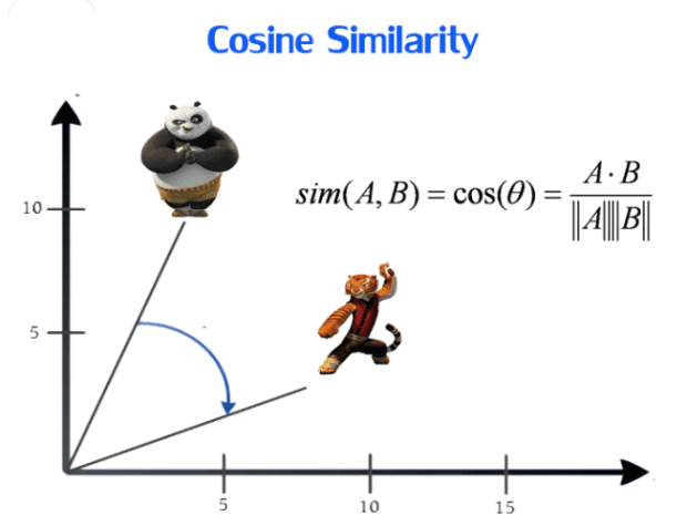
(Cosine similarity; Image from Dataconomy.com)
We use the cosine similarity metric for measuring the similarity of TMT articles as the direction of articles is more important than the exact distance between them. Additionally, we tried both metrics (Euclidean distance and cosine similarity) and the cosine similarity metric simply performs better. 🙂
Two new challenges
Above we described the concept of similarity between articles using a quantified approach. However, now two new challenges arise:
- How can we plot each post in a 2-dimensional space?
- How do we plot these posts such that the distance between the points gives an indication about the similarity of the articles?
An article can be plotted in a 2-dimensional space by assigning it coordinates, i.e. an x and y coordinate. This means we first need to translate our articles to a numeric format and then reduce it to two values, i.e. the x and y coordinate. Therefore, we are first going to elaborate on a scientific approach to quantify the text in the TMT articles by applying feature extraction.
Note that the feature extraction method we discuss below is specifically designed for dealing with text in TMT articles. You can imagine that if you’re building a content-based recommender for telephones you probably need a different method to translate the properties (content) of telephones to a numerical format.
Converting TMT articles to a numeric format
The TMT articles, consisting of large phrases of words and punctuation, need to be translated to numerical vectors without losing the content of the article in the process. Preferably we also want vectors of a fixed size. Why do we want a fixed size? Recall the 2-dimensional example above. It would be strange to compare a point in a 2 dimensional space to a point in a 100-dimensional space right? Additionally, if we want to say something about the similarity between articles we also need to express them in a similar manner.
To obtain vectors of a fixed size we are going to create features, e.g. measurable article properties. In text analysis a feature often refers to words, phrases, numbers or symbols. All articles can then be measured and expressed in terms of the same set of features, resulting in fixed-size numerical vectors for all articles. The whole process of converting text to numerical vectors is called feature extraction and is often done in three steps: tokenization, counting and weighting.

Example of vectorizing text
Step 1: tokenization
The first step in obtaining numerical features is tokenization. In text analysis, tokenization is described as obtaining meaningful basic units from large samples of text. For example, in physics speed can be expressed in meters per second. In text analysis, large strings of text can be expressed in tokens. These tokens often correspond to words. Therefore, a simple tokenization method to obtain tokens for the sentence I am happy, because the sun shines is by splitting them on whitespaces. This splitting results in seven tokens, i.e. I, am, happy,, because, the, sun, shines. After tokenization it is possible to express the original sentence in terms of these tokens.
This simple tokenization method however provides several new problems:
-
For one, this method does not filter out any punctuation and thus the token
happy,contains a comma at the end. This implies that the tokenhappy,andhappyare two different tokens, although both tokens imply the same word. Therefore, we filter out all types of punctuation, because punctuation is almost never relevant for the meaning of a word in our articles.
Note that punctuation can be relevant in other situations. For example, when analyzing Twitter messages punctuation can be important as they are often used to create smiley’s which express a lot of sentiment. The smiley example emphasizes the fact that every data source needs its own feature extraction method. -
Second, using the simple tokenization method it is possible to obtain the tokens
worksandworking. However, these tokens are just different forms of the same word, i.e.to work. The same argument holds for tokens where one is the plural form of the other. For our content-based recommendation system, we assume that both forms of these words imply the same word. Therefore, the tokens can be reduced to their stem and used as a single token. To do this, a stemming algorithm that reduces every word to its stem is required. Note that such a stemming algorithm is language specific. Luckily there are several freely available packages such as theNLTKlibrary that can do this for us. -
A third problem that typically occurs in text analytics is how to deal with combinations or negations of words. For example, just using the individual tokens
GoogleandAnalyticsmay not always imply that we are talking about the productGoogle Analytics. Therefore, we also create tokens of two or three consecutive words, called respectively bi-grams and tri-grams. The sentenceI like big datathen translates to the tokensI,like,big,data,I like,like big,big data,I like bigandlike big data.
Note that this tokenization method does not take into account the position and the order of the words. For example, after tokenization it cannot be said at what position in the original sentence or article the token big occurred. Also, the token itself does not mention anything about the words in front or after it. Therefore, we lose some information about the original sentence during tokenization. The art is to capture as much information about the original sentence while retaining a workable set of tokens.
In our tokenization method we lose information about the structure of the sentences. There are other tokenization methods which take the position and order of words into account as well. For example, Part-Of-Speech (POS) tagging also adds additional information such as the word-class of a token, e.g. whether a token occurs as a verb, adjective, noun or direct object. However, we assume that POS tagging does not greatly increase the performance of our recommender because the order of words within sentences is not of great importance for making recommendations.
Step 2: token frequency counts
In the second step, the frequency of each token in each article is counted. These frequencies are used in the next step for assigning weights to tokens in articles. Additionally these counts are used to later on perform a basic feature selection, i.e. to reduce the number of features. Note that a typical property of text analysis is that the majority of the tokens are only used in a couple of articles. Therefore, the frequency of most tokens in an article is zero.
Step 3: token weights
In the last step the tokens and token frequency counts from the previous steps are used to convert all articles to a numerical format. This is done by encoding each article to a numeric vector whose elements represent the tokens from step 1. Moreover, a token weighting procedure is applied using the frequency counts from step 2. After a token is weighted, it is not any more referred to as a token but as a feature. Hence, a feature represents a token and the value of a feature for an article is a weight assigned by a weighting method.
There are several possible feature weighting methods:
-
The most basic weighting method is Feature Frequency (FF). FF simply uses the frequency of a token in an article as the weight for a token. For example, given the token set {mad, happy}, the sentence
I am not mad, but happy, very happyis weighted as the vector [1 2]. -
Feature Presence (FP) is a similar basic weighting method. In FP the weight of a token is simply given by a binary variable which is 1 if the token occurs in an article and 0 otherwise. The sentence from the previous example would be represented as the vector [1 1] when using FP, because both tokens are present in this sentence. An additional advantage of FP as weighting method is that a binary dataset is obtained, which does not suffer scaling problems. The latter can occur in algorithms when for example calculating complicated values such as eigenvalues or Hessian.
-
A more complex feature weighting procedure is the Term Frequency and Inverse Document Frequency’ (TF-IDF) weighting method. This method uses two scores, i.e. the
term frequencyscore and theinverse document frequencyscore. The term frequency score is calculated by taking the frequency of a token in an article. The inverse document frequency score is calculated by the logarithm of dividing the total number of articles by the number of articles in which the token occurs. When multiplying these two scores, a value is obtained that is high for features that occur frequently in a small number of articles, and is low for features that occur often in many articles.
For our content-based recommendation system we are going to use the FP weighting method because it is fast and does not perform worse than the other weighting methods. Additionally, it results in a sparse matrix which has additional computational benefits.
Reducing the dimensionality
After applying the above feature recommendation method we are left with a list of features with which we can numerically express each TMT article. We could calculate the similarity between each article in this very high dimensional space but we prefer not to. Features that barely express similarity between articles, such as is and a, can be removed from the feature set to significantly reduce the number of features and to improve the quality of the recommendations. Additionally, a smaller dataset improves the speed of the recommendation system.
Document Frequency (DF) selection is the simplest feature selection method to reduce dimensionality and is a must for many text analysis problems. We first remove the most common English stop words, e.g. the words the, a, is, et cetera, which do not give much information about the similarity between articles. After that, all features with a very high and very low document frequency are removed from the data set as these features are also not likely to help in differentiating articles.
Recall that at the beginning of this article we visualized the articles in a 2-dimensional space. However, after applying DF we are still in a very high dimensional space. Therefore we are going to apply an algorithm that reduces the high dimensional space to the 2-dimensional space in which we can neatly visualize the articles. Moreover, it is much easier to understand how the principle of recommendation systems work in a 2-dimensional space as the distance concept then intuitively works well. The algorithm that we use to bring us back to the 2-dimensional space is Singular Value Decomposition (SVD). A different algorithm one can use is Principal Component Analysis (PCA). We do not extensively explain in this article how these algorithms work. In short though, the essence of both is to find the most meaningful basis with which we can reconstruct the original dataset and capture as much of the original variance as possible. Fortunately, scikit-learn already has a built-in version of SVD and PCA which we can therefore easily use.
There are more methods to reduce the dimensionality such as the Information Gain and Chi Square criterion or Random Mapping but for sake of simplicity we stick to the DF feature selection method and PCA dimensionality reduction method.

An example of SVD for dimensionality reduction on the Iris dataset. SVD is applied to reduce the dimensionality from 3D to 2D without losing much information.
Making recommendations
After we have applied all of the above we reduced all TMT articles to coordinates in a 2-dimensional space. For any article we can now calculate the distance between the two coordinates. The only thing we still need is a function that given the current article as input returns a fixed number of TMT articles that have the lowest distance to this article! Using the Euclidean distance formula this function is trivial to write.
Let’s run some scenarios to test our content-based recommender. Suppose we are a user who just finished reading the article Caching $http requests in AngularJS. Our content-based recommender system provides the following TMT article suggestion for follow-up: Angular 2: Where have my factories, services, constants and values gone?. Sounds reasonable, right? The table below provides the results of more scenarios.
| Current article | Recommendation |
|---|---|
| Caching $http requests in AngularJS | Angular 2: Where have my factories, services, constants and values gone? |
| Track content performance using Google Analytics Enhanced Ecommerce report | How article size helps you understand your content performance |
| Data collection and strange values in CSV format | Calculating ad stocks in a fast and readable way in Python |
| How npm 3 solves WebStorm’s performance issues | Webstorm 10 improves the performance of file indexing |
Final remarks
We would like to conclude with a few remarks about our first steps in content-based recommendation systems:
- In our final recommendation system we used SVD to reduce the dimensionality to 30 features instead of 2. This was done because too much information about the features was lost when we reduced it to a 2-dimensional space. Therefore, the similarity metric of articles was also less reliable. We only used the 2-dimensional space for visualization purposes.
- We also applied feature extraction on the title and tags of the TMT articles. This drastically improved the quality of the recommendations.
- The parameters in our recommendation system were chosen intuitively and are not optimized. This is something for a future article!
We hope you learned a few things from this article! Moreover, if you liked this article we recommend to continue reading on TMT with Optimizing media spends using S-response curves… a shameless attempt to improve my author value on TMT. 😉


Leave a Reply
You must be logged in to post a comment.