The science of campaign optimization was among the very first things I was introduced to when first coming to work in programmatic media at Bannerconnect, and it was with great interest that I learned the particular steps our campaign managers regularly take to ensure campaigns run in the most effective way for their advertiser.

Statistically sound optimization

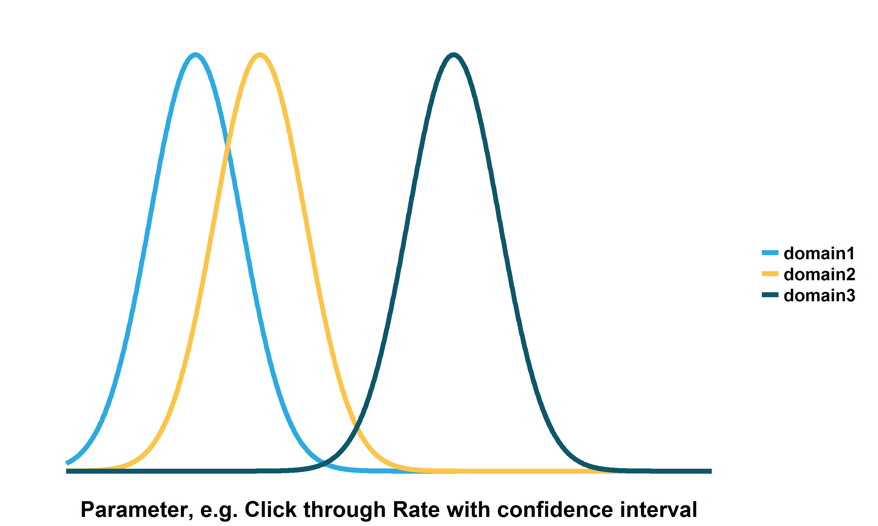
From the data scientist point of view, I was of course very interested in the statistics behind how a certain domain, creative type, or even time of day could be judged to be better than any of the others. When optimizing toward clicks, view times, landings, or final conversions, the answer to the above seems simple enough – there are many types of comparative analysis that one could do between different variable types, and indeed a confidence interval for this binomial type data can be easily calculated, with the resulting confidence interval being largely dependent on the sample size present. The below image visualizes this: domain 2 may appear better than domain 1, but with overlapping confidence intervals, we cannot be sure that there is a real difference.

The difficulty with ratios

However, I quickly came across a more interesting problem: how do you calculate the confidence interval of a ratio of two populations, where there is an uncertainty in each population? For example, what is the confidence interval in my Cost per Action (CPA), given that both the Cost of an impression has a natural variation when taken over a large dataset (and can be presumed to be normally distributed), and the “Action” will also have an uncertainty related to its sample size, and should be binomially distributed? What is the best way to combine these two uncertainties in my measurements, to have a good estimate of how much faith I can put in my calculated CPA?

Previous work in health economics

A quick Google here revealed that not only was I the only one struggling with this problem, but that it was actually more complicated than I had thought. My literature review led me to a different field entirely – that of epidemiology and health economics, where the similar problems had been explored, ignored, or criticized, in turn.

This problem comes about in health economics in the form of cost effectivity ratios – the calculation of how much a treatment costs, versus how likely it is to work. As noted in the paper of Polsky et. al (1), methods for calculating the confidence interval in these ratio are less well developed in their field, and as such often left out of publications. Their work gives a comparison of the effectivity of four methods of calculating these intervals, judging them by performing a Monte Carlo experiment. Of the methods they explore, I’ll mention here only the two which they found most accurate: Fieller’s Method, and a Bootstrap method.

Fieller’s Method

Fieller’s method was first published in 1954, and provides an analytical method for calculating the confidence interval of two ratios, where each part of the ratio may be from a different distribution, i.e. have unrelated uncertainties (2). While this method is very successful for the health economics field, unfortunately for us, it has some conditions which make it inaccurate for the calculation of our CPA, for example. The main restriction that is violated here is that of normality: our “Action” data here will fail this requirement. Another difficulty to be aware of here is that the proportion of positive actions we have in forming our CPA will be extremely low – often less than 1%, which will lead to difficulties in the calculation – a problem that is uncommon in the health field.

Bootstrapping

Happily, the second of the recommended methods they mention, Bootstrapping, leads to much more success. Bootstrapping, simply put, is a method for estimating an estimator (for example the standard deviation), using resampling with replacement of your data. In simple terms, what this means for our example is that we should use a large amount of input data, consisting of cost per impression, and whether the impression resulted in a conversion or not. We can then take a sample of some of these rows, to calculate the CPA. By calculating this thousands of times over different samples of our input data, the distribution of the CPA can be built up, from which we could, for example calculate a standard deviation. While this can sound fiddly, in practice there are bootstrapping routines built into many popular programmes – for example R, SciPy, and MatLab, to name a few.

Armed with these methods, calculating confidence intervals for ratios with unrelated errors becomes much easier, and most importantly, campaign optimizations can be made on statistically sound information!

(1) Polsky, Glick, Willke, and Schulman, “Confidence intervals for cost-effectiveness ratios: A comparison of four methods”, Health Economics, Vol 6: 243-252 (1997).

(2) Fieller, “Some Problems in Interval Estimation”, Journal of the Royal Statistical Society, Series B (Methodological), Vol. 16, No. 2 (1954), 175-185.